Prototypical Network
Prototypical Network (PN) 利用支持集中每个类别提供的少量样本, 计算它们的嵌入中心,作为每一类样本的原型 (Prototype), 接着基于这些原型学习一个度量空间, 使得新的样本通过计算自身嵌入与这些原型的距离实现最终的分类。
1 PN
在 few-shot 分类任务中, 假设有 \(N\) 个标记的样本 \(S=\left(x_{1}, y_{1}\right), \ldots,\left(x_{N}, y_{N}\right)\) , 其中, \(x_{i} \in\) \(\mathbb{R}^{D}\) 是 \(D\) 维的样本特征向量, \(y \in 1, \ldots, K\) 是相应的标签。 \(S_{K}\) 表示第 \(k\) 类样本的集合。
PN 计算每个类的 \(M\) 维原型向量 \(c_{k} \in \mathbb{R}^{M}\) , 计算的函数为 \(f_{\phi}: \mathbb{R}^{D} \rightarrow \mathbb{R}^{M}\) , 其中 \(\phi\) 为可学习参数。 原型向量 \(c_{k}\) 即为嵌入空间中该类的所有 支持集样本点的均值向量
给定一个距离函数 \(d: \mathbb{R}^{M} \times \mathbb{R}^{M} \rightarrow[0,+\infty)\) , 不包含任何可训练的参数, PN 通过在嵌入空间中对距离进行 softmax 计算, 得到一个针对 \(x\) 的样本点的概率分布
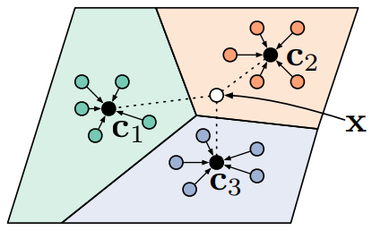
新样本点的特征离类别中心点越近, 新样本点属于这个类别的概率越高; 新样本点的特征离类别中心点越远, 新样本点属于这个类别的概率越低。
通过在 SGD 中最小化第 \(k\) 类的负对数似然函数 \(J(\phi)\) 来推进学习
PN 示意图如图1所示。
2 PN 算法流程
Input: Training set \(\mathcal{D}=\left\{\left(\mathbf{x}_{1}, y_{1}\right), \ldots,\left(\mathbf{x}_{N}, y_{N}\right)\right\}\), where each \(y_{i} \in\{1, \ldots, K\}\). \(\mathcal{D}_{k}\) denotes the subset of \(\mathcal{D}\) containing all elements \(\left(\mathbf{x}_{i}, y_{i}\right)\) such that \(y_{i}=k\).
Output: The loss \(J\) for a randomly generated training episode.
select class indices for episode: \(V \leftarrow \text { RANDOMSAMPLE }\left(\{1, \ldots, K\}, N_{C}\right)\)
for \(k\) in \(\left\{1, \ldots, N_{C}\right\}\) do
select support examples: \(S_{k} \leftarrow \text { RANDOMSAMPLE }\left(\mathcal{D}_{V_{k}}, N_{S}\right)\)
select query examples: \(Q_{k} \leftarrow \text { RANDOMSAMPLE }\left(\mathcal{D}_{V_{k}} \backslash S_{k}, N_{Q}\right)\)
compute prototype from support examples: \(c_k \leftarrow \frac{1}{N_{C}} \sum_{\left(\mathbf{x}_{i}, y_{i}\right) \in S_{k}} f_{\phi}\left(\mathbf{x}_{i}\right)\)
end for
\(J \leftarrow 0\)
for \(k\) in \(\left\{1, \ldots, N_{C}\right\}\) do
for \(x, y\) in \(Q_{k}\) do
update loss \(\left.J \leftarrow J+\frac{1}{N_{C} N_{Q}}\left[d\left(f_{\phi}(\mathbf{x}), \mathbf{c}_{k}\right)\right)+\log \sum_{k^{\prime}} \exp \left(-d\left(f_{\phi}(\mathbf{x}), \mathbf{c}_{k^{\prime}}\right)\right)\right]\)
end for
end for
其中,
\(N\) 是训练集中的样本个数;
\(K\) 是训练集中的类个数;
\(N_{C} \leq K\) 是每个 episode 选出的类个数;
\(N_{S}\) 是每类中 support set 的样本个数;
\(N_{Q}\) 是每类中 query set 的样本个数;
\(\mathrm{RANDOMSAMPLE}(S, N)\) 表示从集合 \(\mathrm{S}\) 中随机选出 \(\mathrm{N}\) 个元素。
3 PN 分类结果
Model |
Dist. |
Fine Tune |
5-way 1-shot |
5-way 5-shot |
20-way 1-shot |
20-way 5-shot |
|---|---|---|---|---|---|---|
MATCHING NETWORKS |
Cosine |
N |
98.1 \(\%\) |
98.9 \(\%\) |
93.8 \(\%\) |
98.5 \(\%\) |
MATCHING NETWORKS |
Cosine |
Y |
97.9 \(\%\) |
98.7 \(\%\) |
93.5 \(\%\) |
98.7 \(\%\) |
NEURAL STATISTICIAN |
- |
N |
98.1 \(\%\) |
99.5 \(\%\) |
93.2 \(\%\) |
98.1 \(\%\) |
MAML |
- |
N |
98.7 \(\%\) |
99.9 \(\%\) |
95.8 \(\%\) |
98.9 \(\%\) |
PROTOTYPICAL NETWORKS |
Euclid. |
N |
98.8 \(\%\) |
99.7 \(\%\) |
96.0 \(\%\) |
98.9 \(\%\) |
Model |
Dist. |
Fine Tune |
5-way 1-shot |
5-way 5-shot |
|---|---|---|---|---|
BASELINE NEAREST NEIGHBORS |
Cosine |
N |
28.86 \(\pm\) 0.54 \(\%\) |
49.79 \(\pm\) 0.79 \(\%\) |
MATCHING NETWORKS |
Cosine |
N |
43.40 \(\pm\) 0.78 \(\%\) |
51.09 \(\pm\) 0.71 \(\%\) |
MATCHING NETWORKS (FCE) |
Cosine |
N |
43.56 \(\pm\) 0.84 \(\%\) |
55.31 \(\pm\) 0.73 \(\%\) |
META-LEARNER LSTM |
- |
N |
43.44 \(\pm\) 0.77 \(\%\) |
60.60 \(\pm\) 0.71 \(\%\) |
MAML |
- |
N |
48.70 \(\pm\) 1.84 \(\%\) |
63.15 \(\pm\) 0.91 \(\%\) |
PROTOTYPICAL NETWORKS |
Euclid. |
N |
49.42 \(\pm\) 0.78 \(\%\) |
68.20 \(\pm\) 0.66 \(\%\) |